Why Our Food Prep Time Prediction Works Better

Our prediction model improves upon estimates from delivery companies by leveraging additional prep state transitions.

This post was written by Zhuyi Xue and Suming J. Chen, who led the development of prep time prediction.

Accurate food prep time prediction has a variety of use cases for food delivery orders. For instance, delivery service providers (DSPs) like UberEats and Doordash need prep time prediction in order to provide estimates for when food will be delivered to their customers, and to better determine when to dispatch couriers to pick up the food. While DSPs have been routinely predicting food prep time, CloudKitchens has an advantage in such prediction because we have more comprehensive insight into kitchen operations. We have deployed our own prep time prediction model that has led to more streamlined logistics (i.e. customers get fresher food and couriers wait less) and fewer customer complaints. 

In this post, we show how we predict prep time for kitchens at CloudKitchens facilities and describe the engineering challenges and product decisions made throughout the process.

Food prep time prediction

Problem Description

For each order, kitchens are required to send prep estimates to DSPs. These estimates are not only used by DSPs, but also by internal facility staff to coordinate logistics. Initially, this value was manually set and usually fixed (e.g. 0/5/10 minutes) – regardless of how busy the kitchen is or what items the order consists of, leading to logistics inefficiencies and customer complaints.

Intuitively, we know how long an order takes to complete depends on a variety of factors (kitchen busyness, order size), but it’s not feasible for kitchen staff to accurately and consistently provide order-specific prep time estimates.

At CloudKitchens, we have valuable kitchen data – real-time monitoring of every kitchen’s current orders-in-progress as well as when each order is complete. Leveraging this data allows us to develop a machine learning (ML) solution to predict the prep time that significantly outperforms heuristic approaches.

Methodology

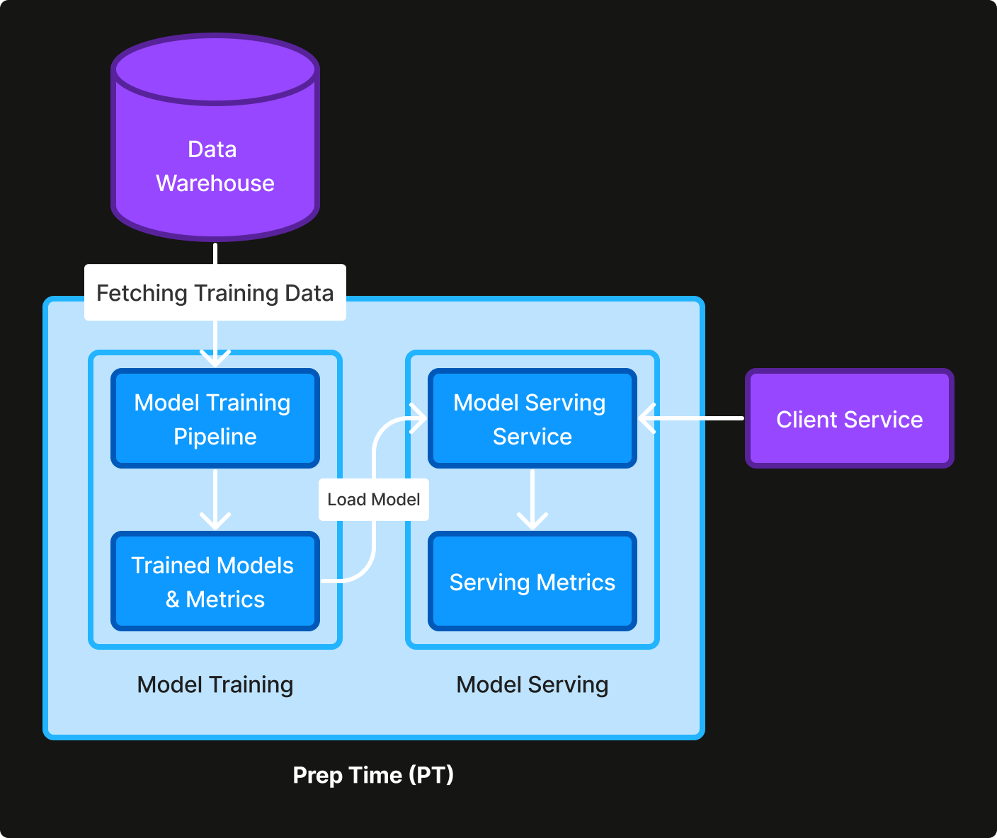
Following the best practices for ML engineering, we did not adopt a ML solution right away at the beginning, and instead just used the median prep time of historical data as the prediction for each kitchen to ensure the infrastructure (e.g. training pipeline, gRPC service, metrics, monitoring) was set up correctly (Figure 1).

Figure 1: Architecture of the prep time model, for both model training and serving.

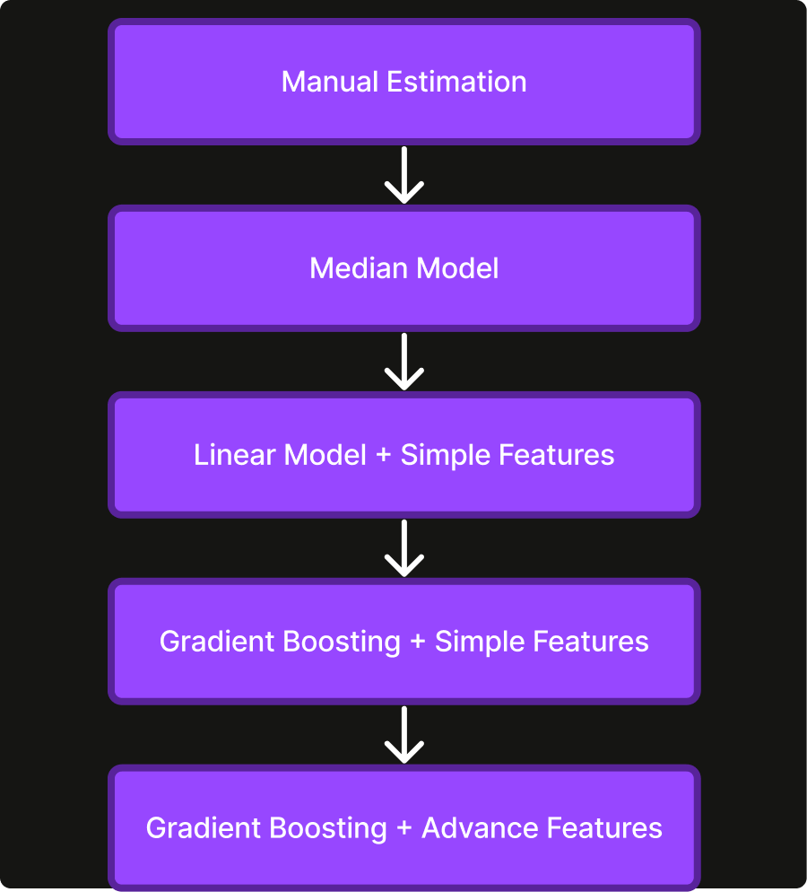
After an end-to-end heuristic model was deployed, we then switched to a linear model with a set of simple features that can be derived from the order itself, e.g. number of items in the order, subtotal of the order, time-of-day of the order. Following, we moved onto a gradient boosting model using LightGBM. We chose LightGBM for its specific way to handle categorical features (e.g. kitchen ID), which tends to outperform one-hot-encoding-based approaches. We also tried a neural network model, but it did not outperform gradient boosting in our experiment, so we decided to shift focus to engineering more advanced features. 

A couple of such features that improve model performance significantly are

1. Average prep time of trailing orders (avg_trailing_prep_time) for a kitchen. The trailing orders are the most recently completed orders before the order we’re predicting prep time for.

2. Total number of orders being currently prepared from all DSPs in the kitchen (num_queued_orders), a proxy for kitchen busyness. 

Both features are available to CloudKitchens kitchens but hidden from DSPs. What distinguishes them from the simple features is that they’re highly dynamic as they depend on the states of other orders from the same kitchen. The avg_trailing_prep_time feature needs to be updated whenever an order is finished cooking and the num_queued_orders feature needs to be updated whenever a new order comes in or an existing order is finished cooking. Such dynamic nature poses challenges to ensure feature consistency between model training and serving times, which will be further discussed in the Engineering Challenges section.

Figure 2. Progression of model and feature complexity.

As we progress towards more complex models and features (Figure 2), model performance consistently improves. Compared to the manual predictions, our ML-based solution improves the mean absolute error (MAE) by 42%. We choose MAE over mean squared error (MSE) as the main metric for its robustness against outliers.

Engineering challenges

Feature consistency

The calculation of features like avg_trailing_prep_time and num_queued_orders requires tracking of all recent order states in a kitchen. Initially, at training time, we calculated such features in Python, while at serving time, the model client was written in Java. As a result, the same logic was implemented twice in different languages, which almost always led to some feature skew between training and serving time, and was unscalable for adding additional features.

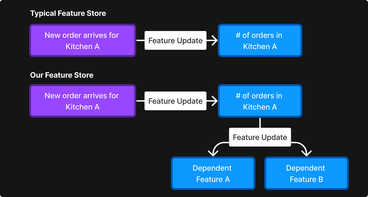
To deal with the feature skew issue, we decided to use a feature store. We evaluated multiple open-source solutions for feature store implementations, but found that there were drawbacks to each approach, e.g. they could not integrate with the multi-regional technologies CloudKitchens uses, or their lack of support in SDK for our stack.

In addition, we recognized the need for a system that could handle the complex interdependencies between various data features due to their highly dynamic nature. Specifically, we required a setup where an update to one feature could automatically trigger updates to related features across different entities. For example, when a kitchen completes an order faster than anticipated, this event could alter our prediction of preparation times for pending orders in that kitchen, which might also affect the kitchen's direct-to-consumer ranking, which is also considered a feature, compared to others. To address this, we built our own feature store using CockroachDB (Figure 3), which was chosen for its resiliency and scalability. This feature store was designed to support the cascading updates of feature values that our data environment demanded. 

Figure 3. A typical event-drive feature store versus the feature store we built.

Automatic model refresh

As CloudKitchens expands rapidly, new kitchens continue to be added, so the prep time model needs to be retrained periodically with the most recent data to account for them. In addition, the evolution of prep time patterns in existing kitchens driven by events like cooking appliance upgrades/additions, menu updates, and staff churn also requires periodic model refreshes.

To make model refresh scalable to additional logistics models, we implemented an automatic model refresh strategy (Figure 4). Suppose the incumbent model (M_i) is trained on data between t₀ and t₃, and some new data is collected between t₃ and t₅. To train and evaluate a new model, we follow these steps:

1. Split the data between t₁ and t₅ into three parts: fit set (t₁-t₂), validation set (t₂-t₄), test set (t₄-t₅). Note, we keep t₅ - t₃ = t₁ - t₀ to avoid including very old data for model training because our research shows that, contrary to the common impression that the more data the better, they hurt model performance when evaluated on the most recent orders, which indicates that prep time patterns evolve quickly.

2. Fit a model on the fit set, validate it on the validation set, conduct hyperparameter tuning, and pick the best hyperparameters (HP).

3. Train a candidate model for comparison (M_c) on the fit + validation set with HP. 

4. Calculate the metrics for both M_i and M_c on the test set, and compare them.

5. If M_c outperforms M_i, train a new production-ready model M_p on fit + validation + test set with HP.

Figure 4. Vertical arrows indicate timestamps used when designing the auto refresh strategy. Horizontal arrows label the time interval between two timestamps. Rectangles indicate the data used for training the incumbent or the new model.

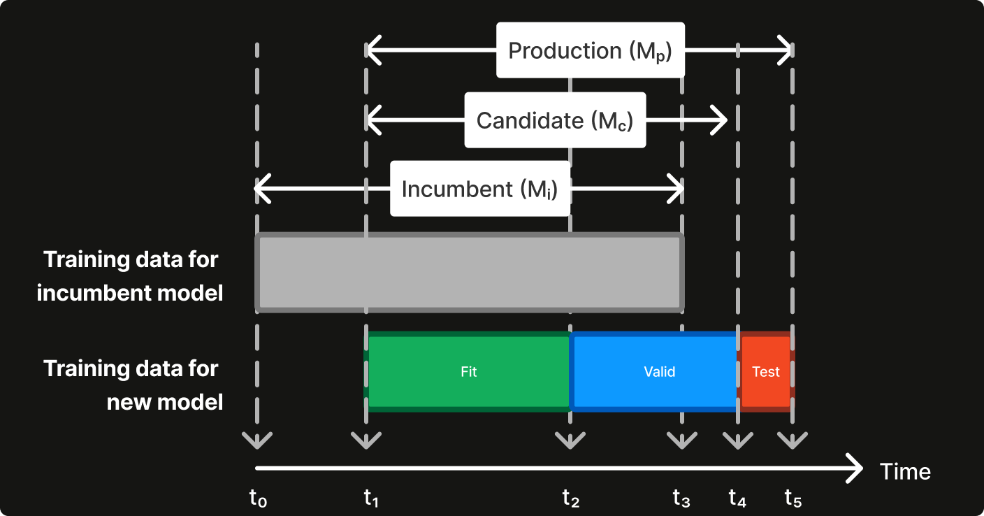
Note, the new data collected between t₃ and t₅ must be split into two parts because 1) if all of it is used for training, then we have no data for testing; or 2) if all of it is used for testing, then the new model can only be trained on the same or a subset of data used for training the incumbent model, and will unlikely show any improvement.

Independent of model training, the model service attempts to load the latest production-ready model in a cron-like fashion so that it can make use of M_p shortly after it becomes available. We also have monitoring in place to alert if the incumbent model gets too old for unexpected reasons.

Product Decisions

Quantile prediction

Some of our products require quantile predictions besides a point estimate of the mean/median prep time. For instance, our decision-making algorithm for deciding when to send a scheduled order to the kitchen for preparation is based on p25 and p75 quantiles of the prep time estimates. To accommodate the additional quantiles, we have opted for quantile regression for model training, which uses a so-called pinball loss:

where t is the ground truth label, x is the feature vector, y is the model, I is the indicator function, and τ ∊ (0, 1) is the alpha corresponding to the quantile interested. When τ = 0.5, pinball loss is equivalent to MAE loss. We evaluate our quantile regression models by checking their average calibrations, e.g. a p25 model should produce predictions that are lower than the ground truth labels about 25% of time. While exploring alternatives, we also considered NGBoost, which generates a probabilistic forecast based on a pre-assumed parametric distribution (e.g. lognormal). However, NGBoost took significantly longer to train a model on our dataset, rendering it less practical. Besides being more scalable, quantile regression offers the advantage of not imposing any assumptions about the distribution form. A drawback of this approach is the need to train separate models for each quantile, so p25, p50 and p75 correspond to three distinct LightGBM models. Given our focus on only a few quantiles, quantile regression remains a suitable choice. We view quantile regression as a compromise between point estimation and fully probabilistic forecasting. 

Remaining prep time prediction

When an order is first received, we always make an initial prep time prediction to return to the DSP. However, our belief in this prep time is fluid, meaning that over time there are events that may change our initial estimate. For instance, we may have initially predicted that an order would take 15 minutes, but 10 minutes into food prep the kitchen may have become much busier, so we would be able to take into account the updated state and make a more accurate prediction for the remaining prep time. Our motivation for this is to ensure that at any point in time, the most accurate estimate is available – important for use cases like planning robot routing for order conveyance as well as keeping couriers updated on the pick up time.

Figure 5. Horizontal bars show prep time of each order. Blue shows the order we are sampling training examples from. Gray shows other orders from the same kitchen. Vertical arrows show the timestamps we sample at, e.g. t1 and t4 are sampled when an existing order is finished cooking, and t2, t3, t5, t6 are examples sampled when a new order is received.

We solve this problem by:

1. Adding an additional feature that measures how much time has passed since an order is received (time_since_order_received). As illustrated in Figure 5,  at t₀, the time_since_order_received is 0, and at t₁, it is t₁ - t₀, and so on.

2. Sampling additional training examples whenever there is a change in kitchen state. An example is sampled whenever a new order arrives (t₂, t₃, t₅, t₆) or an existing order is being completed (t₁, t₄), so seven examples are obtained from the order instead of one in Figure 5. Using the aforementioned feature store, it is straightforward to sample the training data at different timestamps within an order’s prep time. 

   

   Figure 6. Remaining prep time prediction prevents zero or negative prediction.

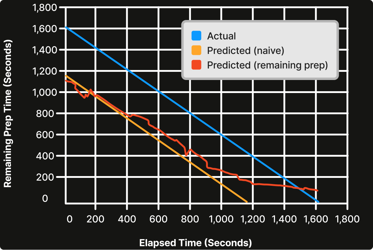
As shown in Figure 6, at any point in time, we could simply estimate the remaining prep time by subtracting the initial predicted prep time (~20min) by elapsed time (orange line). However, we can see that 20 minutes in, the only option is to continually show 0 minutes remaining or show negative numbers. Instead, if the remaining prep time is used, we can continue to finesse the prediction all the way until the order is complete (red line). The remaining prep time model is shown to be 10% more accurate than the baseline approach.

Conclusion

We describe how we leverage the unique data we have in order to predict food prep time 42% more accurately than the naive baseline.  We discuss our approach to engineering challenges like train/serve feature consistency, automatic model refresh, and how we enabled this feature to be even more powerful by adding on quantile predictions and the ability to predict the remaining prep time. In the future, with the addition of new technologies and increased capacity to capture the state of the kitchen, we expect to continue to improve model quality.